From Pixels to Perception: A Technical Guide to Color Analysis in Digital Images

Introduction

Color analysis in digital images has become increasingly crucial in modern software development, from creating adaptive user interfaces to analyzing brand consistency in marketing materials. This comprehensive guide takes you on a journey from understanding basic bitmap principles to implementing sophisticated color analysis techniques using machine learning approaches.

Who This Guide Is For

This guide is designed for:

Software developers working with image processing
Computer science students learning about color analysis
UI/UX designers interested in programmatic color extraction
Anyone curious about how computers understand and process colors

What You’ll Learn

By the end of this guide, you’ll understand:

How digital images store color information
Different approaches to analyzing image colors
Why human color perception matters in software
Advanced techniques for accurate color analysis
When to use different color analysis methods

Prerequisites

Basic programming knowledge (examples use Kotlin)
Understanding of basic computer science concepts
Familiarity with binary operations is helpful but not required

Part 1: Foundations of Digital Images

What is a Bitmap?

Bitmaps represent one of the fundamental ways to store digital image data. In a bitmap, an image is decomposed into a grid of tiny squares called pixels, with each pixel containing information about its color stored in bits. Early computer systems used single-bit pixels, creating monochrome images with just black and white colors. Modern systems have evolved far beyond these limitations, enabling rich color representation and sophisticated image processing capabilities.

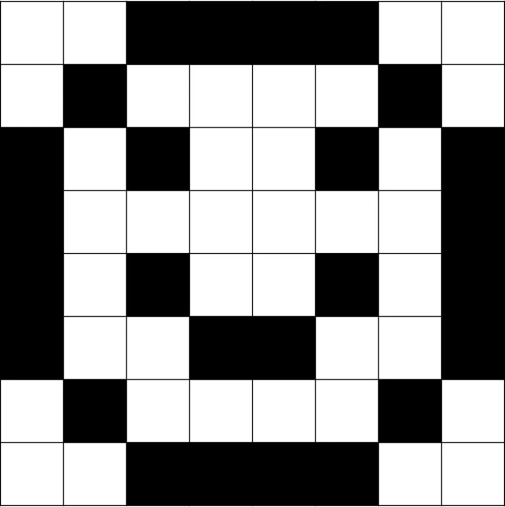
Black and White Bitmap representation (From Harvard CS50)

The computer representation shown above demonstrates how early bitmap systems worked, with each pixel represented by a single bit — 1 for white and 0 for black.

This would result in the following:

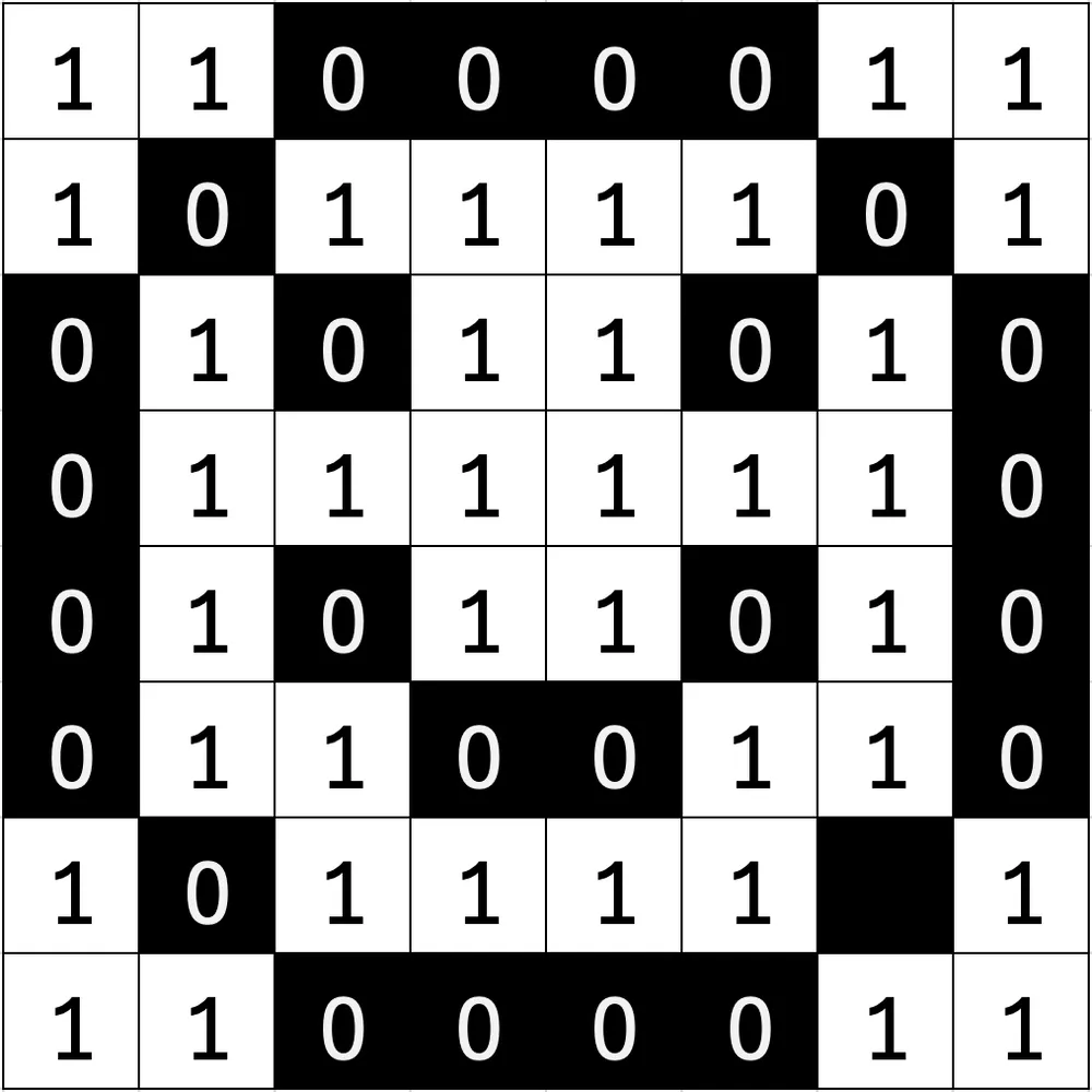
Computer representation of previous Bitmap

Beyond Monochrome

As technology progressed, images started using more bits per pixel, allowing them to represent a wider range of colors and greater image detail. The resolution of a bitmap, measured in dots per inch (dpi), determines the quality of the image — the higher the resolution, the clearer the image appears. Additionally, the color depth, or the number of bits used to represent each pixel’s color, affects how vivid and lifelike the image appears.

Modern images typically use 24-bit color, providing up to 16.7 million colors (2²⁴). This detailed color representation creates higher-quality images but also increases the amount of memory required to store them.

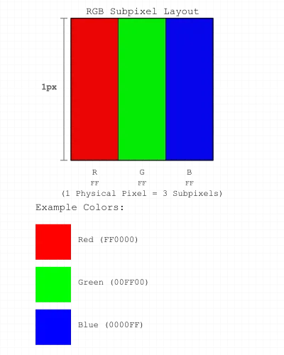
In a 24-bit Bitmap, 8 bits are used for each of the primary colors: red, green, and blue. This is where the term RGB color comes from. The last 8 bits often represent the alpha channel, determining transparency.

24 bit representing a pixel with only red value

If we take the image above as an example, if a pixel’s RGB values are 0xff (255 in decimal) for red, 0x00 for green, and 0x00 for blue, the pixel displays a pure red color, as the high value for red indicates maximum intensity, while the zeros for green and blue show no contribution from those colors.

This creates a vivid red pixel because we’re telling our display “Show full red, but don’t add any green or blue.”

Now, let’s apply this understanding to create a simple face using distinct colors for each feature:

Head: Pure Red (FF0000)

Maximum red, zero green, zero blue

Smile: Pure Green (00FF00)

Zero red, maximum green, zero blue

Eyes: Pure Blue (0000FF)

Zero red, zero green, maximum blue

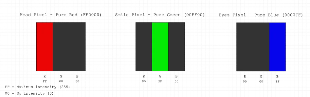
By upgrading from a single-bit (monochrome) to 24-bit colored bitmap, we can now represent over 16 million colors! Each pixel stores three 8-bit values (one each for red, green, and blue), giving us far more expressive power than the original black-and-white version.

The resulting bitmap showcases how these primary colors combine to create our simple yet colorful face, demonstrating the fundamental principles of digital color representation.

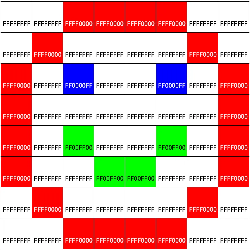
Representation of a 24 bit per pixel bitmap

Bonus: Calculating Bitmap Size

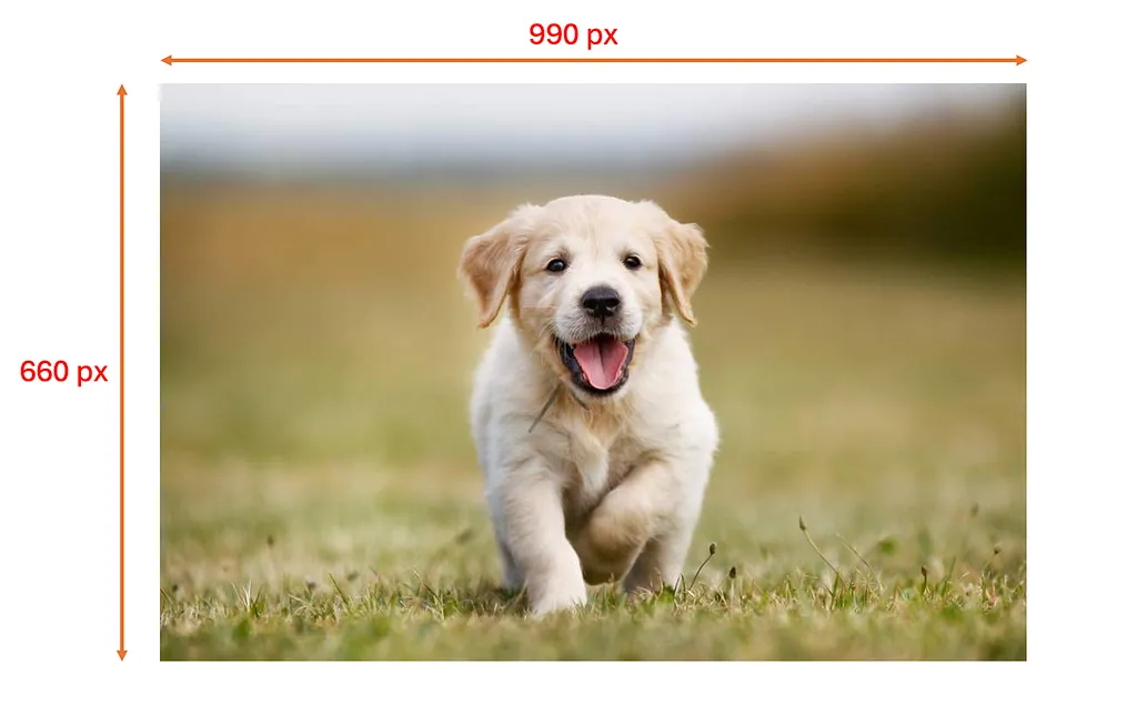
The bitmap grid in this example measures 990 by 660 pixels, meaning there are 990 pixels per row and 660 pixels per column. This results in a total of 990 * 660 = 653,400 pixels.

Since each pixel contains a 24-bit color value, we divide 24 by 8 to convert it to bytes, resulting in 3 bytes per pixel. Therefore, the total size of the bitmap in bytes is:

3 * 653,400 = 1,960,200 bytes.

Next, to convert this into kilobytes, we divide by 1,024:

1,960,200 / 1,024 = 1,914 KB.

Finally, dividing by 1,024 again, we obtain the size in megabytes:

1,914 / 1,024 ≈ 1.86 MB.

It’s important to note that the image file might also contain metadata, such as information about the image’s resolution, color depth, or the device used to capture it. This additional data can increase the file size slightly beyond our calculations.

Part 2: Basic Color Analysis

Finding the Dominant Color in a Bitmap

Now that we have a good understanding of how bitmaps work, let’s explore how to identify the most dominant color within a bitmap. The dominant color is the one that appears most frequently in the image and can help with various tasks such as color palette generation, image sorting, or simply understanding the visual composition of an image.

Why Find the Dominant Color?

Understanding the dominant colors in an image has become increasingly important in modern applications, from user interface design to machine learning systems. The dominant color can inform adaptive theming, content categorization, and even emotional analysis of images.

Traditional Approaches and Their Limitations (Intuitive Solution)

In a bitmap, each pixel has a color value, usually represented in ARGB format. To find the dominant color, we need to:

Scan through each pixel of the image.
Track the frequency of each color in the bitmap.
Determine the most frequently occurring color in the image.

Here’s a Kotlin implementation for code we described:

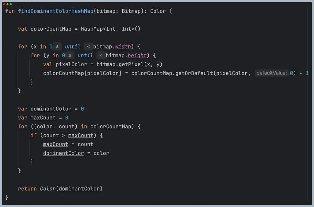
Intuitive Solution using Kotlin

However, scanning through each pixel and counting occurrences for potentially millions of colors can be inefficient, especially with large images. To handle this, we need to choose an effective approach for storing and processing color frequencies, which will be discussed further in Part 3.

Observed Issues

Color Variability: In a 24-bit color space, there are more than 16 million possible colors. Using an exact match for each color (as with a HashMap) means that even minor variations in color (e.g., slight differences in shade) are treated as separate colors. This results in a fragmented color count, making it difficult to accurately determine the dominant color. For example, consider a bitmap containing 100 pixels: 5 pixels are green (`0xFF00FF00`), and the remaining 95 are various shades of blue that are nearly indistinguishable to the human eye. In this case, our current algorithm might incorrectly identify green as the dominant color because it counts every slight variation in blue as a separate color. This approach fails to group similar colors together, leading to an inaccurate representation of the dominant color in the image.
Memory Inefficiency and Overhead: When working with small to medium-sized bitmaps, using a HashMap to count color frequencies can introduce several issues like using extra memory which we will cover in the next part. While lookups are pretty fast, hashing and resizing can introduce some overhead as well.
Some Bitmaps could be Very Large: When analyzing high-color-depth images (24-bit RGB), we face a significant computational challenge. With 16,777,216 possible colors, iterating through every unique color in a HashMap becomes computationally expensive and often unnecessary. For finding dominant colors, we rarely need to analyze the full color space.

In the next section, we will tackle Color Variability and see how we can work on this issue to improve our analysis!

Part 3: Improving Accuracy with Color Bucketing

Color Variability

As we mentioned earlier, directly using the exact pixel colors to find the dominant color can lead to inaccuracies due to slight variations in shades. For example, in an image with multiple shades of blue, each shade might be counted as a unique color, even though they visually appear similar. To address this, we use color bucketing, which groups similar colors together to reduce the number of distinct colors. This helps in identifying a more representative dominant color.

Let’s take the following color and inspect its properties:

Example: Let’s inspect the RGB color RGB(161, 200, 238):

The result indicates that blue dominates due to its high value, we will use this color in the background of the image below:

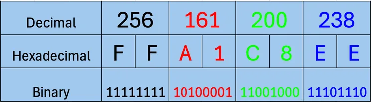
Representation of RGB(161,200,238) color with this color as background

Prerequisites Refresher_
Before we dive into color manipulation, let’s quickly review some key concepts:_

Bitwise Operations:
- Shifting Right (shr): Moves bits to the right, filling with zeros from the left
Example: 1100 shr 2 = 0011
- AND (&): Returns 1 only if both bits are 1
Example: 1100 & 1010 = 1000
- OR (|): Returns 1 if either bit is 1
Example: 1100 | 1010 = 1110

Color Components:
- Each color is stored in 32 bits (4 bytes)
- Format: [Alpha(8 bits)][Red(8 bits)][Green(8 bits)][Blue(8 bits)]
- Each component ranges from 0 to 255 (8 bits = 2⁸ = 256 values)

Extracting Individual Color Components

To separate the red, green, and blue values, we use bitwise manipulation. Since each color component (red, green, blue) occupies 8 bits, we can isolate them with bit shifting.

Step 1: Extracting the Red Value

The blue and green colors occupy the last 16 bits. To isolate the red value, we shift the bits 16 places to the right.
This operation fills the leftmost bits with zeros, giving us a result that contains the red value and the alpha channel.

Shifting Right by 16 ->

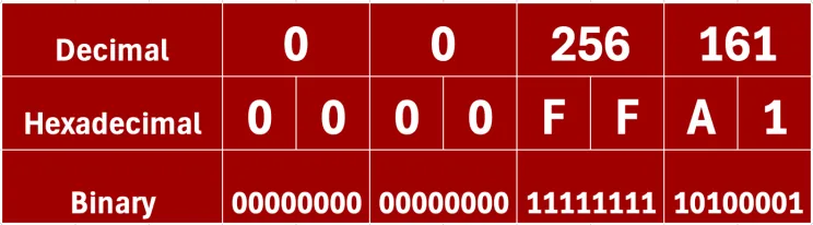
Resulting color with it’s background as the color

Step 2: Removing the Alpha Channel

To extract just the red component, we use the bitwise AND operator:
Reminder:
1 AND 1 = 1
1 AND 0 = 0
0 AND 0 = 0

Applying this operation removes the alpha channel, leaving us with only the red value.

We get the following result:

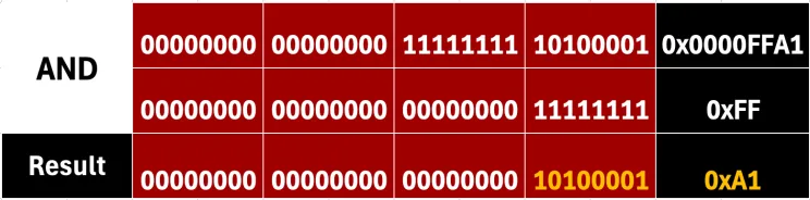
Applying AND bitwise operator

Now, we have successfully extracted the red component: 0xA1.

Extracting the other colors:

Green: Shift the bits by 8 to the right to isolate the green component then apply AND Operator with 0xFF
Blue: No shifting is needed, as the blue value is already in the correct position at the end.

Applying the same the same process gives us the following:

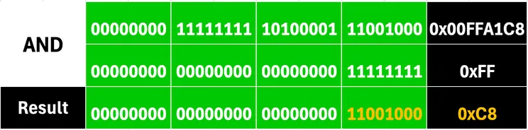
Shift Right by 8 then Apply AND operation

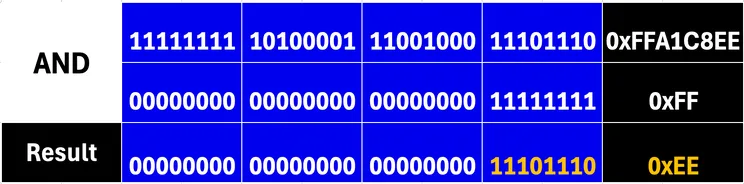
Apply AND operation without Shifting

Kotlin Code Representing what we just did:

val red = (color shr 16 and 0xFF)val green = (color shr 8 and 0xFF)val blue = (color and 0xFF)

Until now, we have separated each color component into its own variable. However, we still need to perform color bucketing to further simplify the color representation.

Color Bucketing

Each color component (red, green, and blue) ranges from 0 to 255, which gives us 256 possible values per channel. To reduce the number of distinct colors, we apply a bucketing process:

Divide by 32: This step reduces the number of possible values for each color channel. The original range of 0 to 255 is divided by 32, resulting in 8 possible values (since 256 / 32 = 8).
Multiply by 32: After dividing, we shift the values back to the nearest multiple of 32. This rounding simplifies the color space by grouping similar colors into fewer buckets.

Example with the Color (161, 200, 238):

Red Component: 161
Green Component: 200
Blue Component: 238

Final Bucketed Color: 160, 192, 224

After applying the bucketing step, the color (161, 200, 238) becomes (160, 192, 224). This simplified color representation reduces the number of distinct colors in the image, making it easier to identify the dominant color by grouping similar shades together.

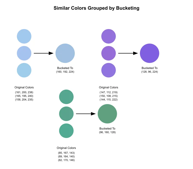
Reconstructing the Color:

Once we have the bucketed values for each color component, we need to combine them into a single 32-bit color integer. In Android, colors are typically represented in the ARGB (Alpha, Red, Green, Blue) format. The ARGB color value is a 32-bit integer where:

The alpha component (opacity) occupies the most significant 8 bits.
The red component occupies the next 8 bits.
The green component occupies the following 8 bits.
The blue component occupies the least significant 8 bits.

To reconstruct the color, follow these steps:

Shift the Alpha Component: Shift Left the alpha bits by 24 bits to be at the start.
Shift the Red Component Shift the red component left by 16 bits to place it after the alpha.
Shift the Green Component: Shift the green component left by 8 bits to place it after the red color.
Combine All Components: Use the bitwise OR operator to combine the shifted components into 1 color.

PS: No need to shift the blue color since it should be placed at the end anyways.

The bucketed color resulting from our original color:

Red: 160 (A0)
Green: 192 (C0)
Blue: 224 (E0)

Performing an OR bitwise operation on all of the bits as follows:

Reminder:

1 OR 1 = 1
1 OR 0 = 1
0 OR 0 = 0

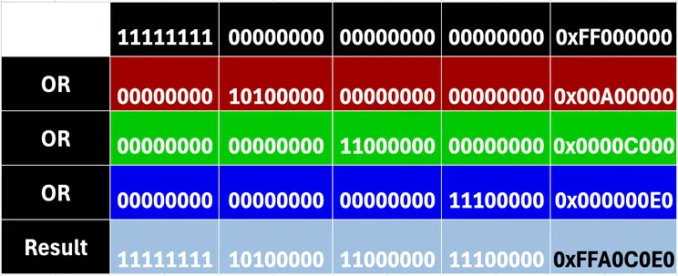
The Kotlin code implementation is as follows:

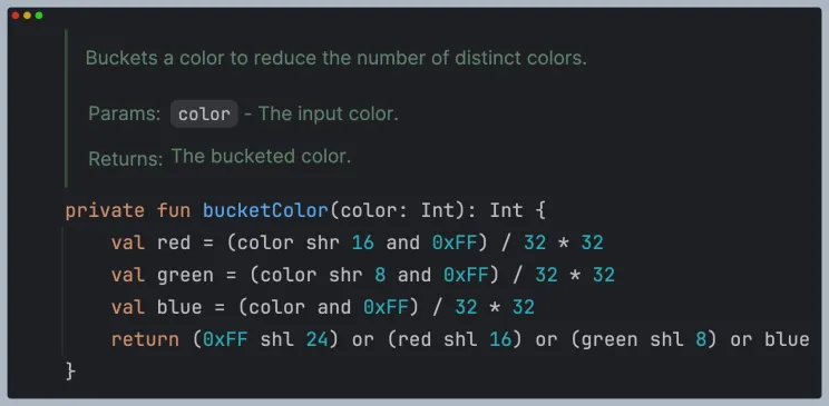
While color bucketing represented a significant improvement over naive color counting, modern applications often require more sophisticated approaches. Nevertheless, understanding bitwise operations remains valuable for low-level image processing tasks. In the next part, we will see how we can further improve our algorithm.

Part 4: Performance Optimization Techniques

With color bucketing in place, we now have a HashMap containing fewer entries, which theoretically speeds up our algorithm and reduces memory usage. However, there are additional optimizations we can apply to further enhance performance and efficiency.

Bitmap Downscaling

Before diving into data structure optimizations, it’s crucial to address the size of the bitmap itself. Processing large bitmaps can be computationally expensive and memory-intensive, especially when iterating over millions of pixels to find the dominant color. However, our goal is to identify the dominant color, not to preserve every pixel’s exact shade. This allows us to downscale the bitmap, significantly reducing the number of pixels to process while maintaining an accurate representation of the overall color composition.

Why Downscale? Downscaling reduces the dimensions of the image, thus reducing the total number of pixels. This makes the color-detection process faster and less memory-intensive. In practice, a smaller image (e.g., 25% of the original size) often provides a sufficiently accurate dominant color for most applications.
How to Downscale: We create a smaller version of the bitmap using a simple scaling function, shrinking its width and height. This is typically done before extracting pixel colors, allowing us to work with a more manageable data set from the outset.

By downscaling the bitmap, we significantly reduce the computational workload, making subsequent processing steps more efficient.

fun downscaleBitmap(original: Bitmap, targetWidth: Int): Bitmap {    val ratio = targetWidth.toFloat() / original.width    val targetHeight = (original.height * ratio).toInt()        return Bitmap.createScaledBitmap(        original,        targetWidth,        targetHeight,        true  // Use bilinear filtering    )}

Nearest Neighbor vs Bilinear Filtering

When downscaling images, we need a method to determine the color values of pixels in our smaller image. Two common approaches are nearest neighbor and bilinear filtering, each with its own characteristics and trade-offs.

Nearest Neighbor Interpolation: This is the simpler approach — imagine shrinking a photo by placing a grid over it and just picking the closest original pixel for each new position. It’s like asking “which original pixel is nearest to where I need a color?” and using that exact color. For example, if we’re halfway between a red pixel and a blue pixel, nearest neighbor will simply choose whichever one is slightly closer, with no blending.

This approach:

Preserves original color values exactly as they appeared in the source image
Can create jagged edges and blocky appearances
Might miss important color variations if a significant color happens to fall between sample points
Is computationally faster since it involves simple position calculations

Bilinear Filtering: This more sophisticated approach considers the surrounding context of each new pixel position. Instead of picking just one nearby pixel, it looks at the four closest pixels and creates a weighted blend based on distance.

Here’s how it works:

For any given output position, identify the four surrounding input pixels. Imagine you’re standing at a point, and there are pixels at the corners of a square around you.
Calculate how far you are from each of these four corners
Use these distances to determine how much each pixel should influence the final color. Closer pixels have more influence than farther ones.
Combine all four colors proportionally to create a smooth blend

For example, if you’re:

Exactly halfway between a red and blue pixel horizontally
The resulting color would be a perfect purple blend
If you’re closer to the red pixel, the result would be a more reddish-purple

This approach:

Creates smoother transitions between colors
Better preserves the overall color distribution of the image
Is more computationally intensive
Is particularly important for color analysis since it maintains a more accurate representation of the image’s color composition

For dominant color detection, bilinear filtering is often the preferred choice despite its higher computational cost, because it provides a more accurate representation of how colors are distributed in the original image. When we’re trying to understand what colors are truly dominant in an image, maintaining these smooth transitions and accurate color relationships is crucial.

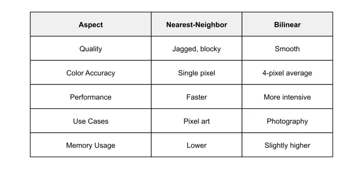
Note: The cost of bilinear filtering is typically minimal and the improved image quality is significant, so using bilinear filtering is often recommended.

Part 5: Advanced Approaches to Color Analysis

Beyond Simple Color Counting

While our earlier approaches of color bucketing worked well for basic analysis, modern applications often need more sophisticated ways to understand colors in images. This brings us to two key improvements: using LAB color space and clustering similar colors together.

Understanding LAB Color Space

When we look at a photo, our eyes naturally group similar colors together. But computers see colors differently — they work with RGB values that don’t match how humans perceive color differences. This is where LAB color space comes in.

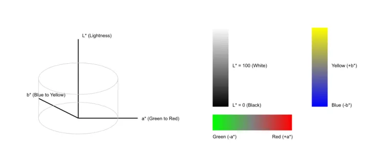
LAB color space has three components that better match human vision:

LAB color representation

L* (Lightness): Think of this as how bright a color is, from black (0) to white (100)
a*: This shows how red or green a color is
b*: This shows how blue or yellow a color is

The magic of LAB space is that equal distances between colors match what our eyes see as equal differences. This is crucial for our next step — grouping similar colors together.

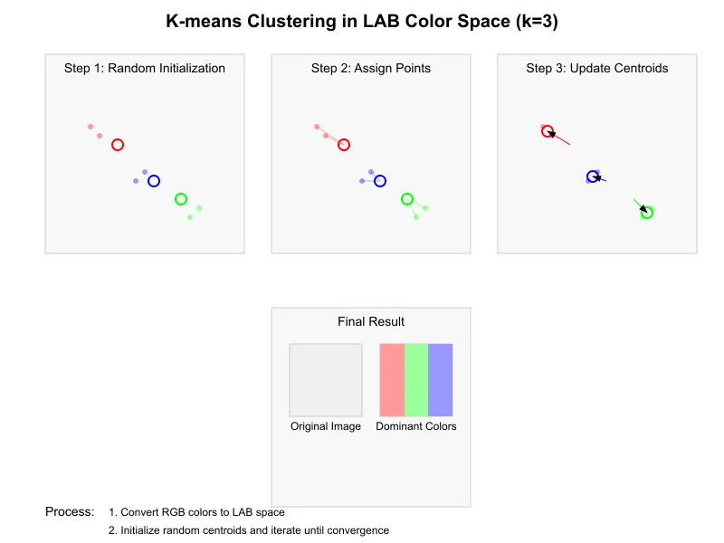
K-means clustering

Color Clustering

Teaching computers to group colors like humans.

Imagine sorting a box of colored marbles. You’d naturally group similar shades together — all the reddish ones in one pile, bluish ones in another. This is exactly what our clustering approach does with image colors.

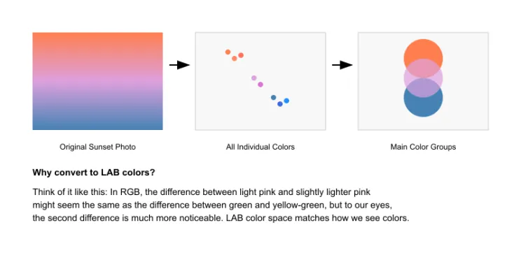
Before starting our process, we should convert image colors to LAB space (giving the computer “human-like” color vision)

The process, called k-means clustering, works like this:

Decide how many color groups we want (let’s say k=3 for a sunset photo)

The computer then :

Looks at all the colors
Groups similar ones together
Finds the average color for each group
Keeps refining these groups until it has the best grouping

When Should You Use This Approach?

Perfect for:

Creating color palettes from images
Finding theme colors for user interfaces
Analyzing artwork’s color composition
Brand color analysis

Not ideal for:

Quick color checks (is an image mostly dark?)
Real-time processing (like video)
Memory-constrained environments
Simple dominant color detection

Clustering LAB colors gives us results that match what humans would naturally choose as the main colors in an image. While this approach takes more processing power than simple color counting, it provides much more accurate and useful results for applications where human perception matters.

This implementation offers several advantages:

Performance Optimization: The sampling step reduces processing time while maintaining accuracy.
Accurate Color Representation: K-means naturally handles color variations and produces representative colors.
Flexibility: The algorithm can be adjusted to find any number of dominant colors.

Practical Applications

Adaptive UI Theming: Applications can dynamically adjust their color schemes based on content.
Image Organization: Large image collections can be automatically categorized by color palette.
Content Analysis: Color patterns can inform emotional analysis of images or brand consistency checking.
Accessibility: Dominant colors can be analyzed for contrast ratios to ensure readability.

When to Use Different Approaches

Your choice of color analysis method should depend on your specific needs:

For Quick Analysis (Simple Color Counting):

Real-time color presence detection
Basic color distribution analysis
When each pixel colors matter

For Efficient Analysis (Color Bucketing):

Dark/light ratio determination
Memory-efficient color analysis
When similar colors can be grouped
Basic color categorization
When precision isn’t critical

For Professional Results (LAB + Clustering):

Color-critical applications
When human perception accuracy matters
Professional palette extraction
Fine art and photography analysis
When subtle differences matter

The Future of Color Analysis

As machine learning and computer vision continue to advance, we’re seeing new approaches emerge:

Deep learning models that understand color context
Real-time color analysis for video streams
Color-based emotion detection in images
Automated accessibility checking for color combinations

Conclusion

The journey from simple pixel counting to sophisticated color analysis reflects the broader evolution of image processing. While simpler approaches like color bucketing still have their place, understanding advanced techniques like LAB color space and clustering enables us to create applications that better match human perception.

Whether you’re building an adaptive UI system, organizing an image collection, or analyzing brand consistency, the concepts and techniques in this guide provide a solid foundation for implementing effective color analysis in your applications.

Remember that the best approach often depends on your specific needs — sometimes a simple solution is perfect, while other times the extra computational cost of advanced methods is worth the improved accuracy.